Gathering Data
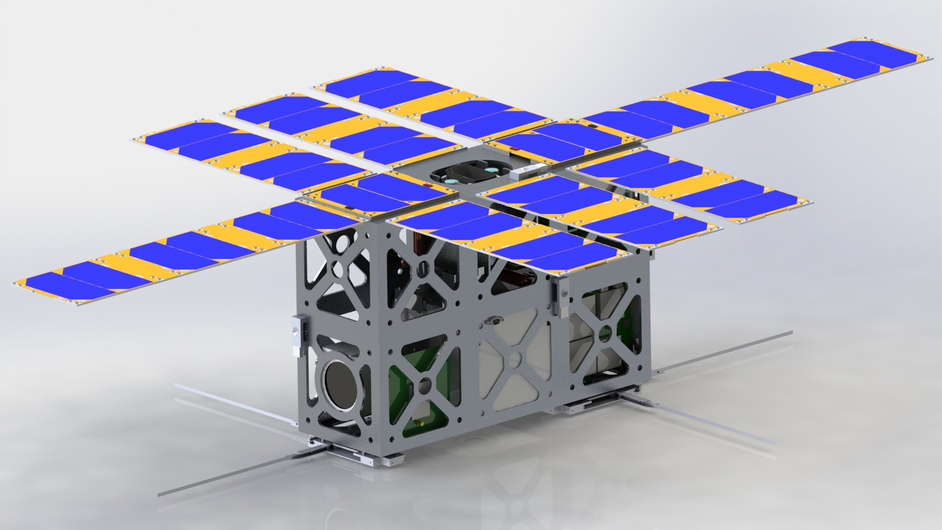
To get started on the project before any scans of the actual debris are made available, I opted to find 3D models online and process them as if they were data collected by my team. GrabCAD is an excellent source of high-quality 3D models, and all the models have, at worst, a non-commercial license making them suitable for this study. The current dataset uses three separate satellite assemblies found on GrabCAD, below is an example of one of the satellites that was used.
Data Preparation
The models were processed in Blender, which quickly converted the assemblies to stl files, giving 108 unique parts to be processed. Since the expected final size of the dataset is expected to be in the magnitude of the thousands, an algorithm capable of getting the required properties of each part is the only feasible solution. From the analysis performed in Report 1, we know that the essential debris property is the moments of inertia which helped narrow down potential algorithms. Unfortunately, this is one of the more complicated things to calculate from a mesh, but thanks to a paper from (Eberly 2002) titled Polyhedral Mass Properties, his algorithm was implemented in the Julia programming language. The current implementation of the algorithm calculates a moment of inertia tensor, volume, center of gravity, characteristic length, and surface body dimensions in a few milliseconds per part. The library can be found here. The characteristic length is a value that is heavily used by the NASA DebriSat project (Murray et al. 2019) that is doing very similar work to this project. The characteristic length takes the maximum orthogonal dimension of a body, sums the dimensions then divides by 3 to produce a single scalar value that can be used to get an idea of thesize of a 3D object.

The algorithm’s speed is critical not only for the eventual large number of debris pieces that have to be processed, but many of the data science algorithms we plan on performing on the compiled data need the data to be normalized. For the current dataset and properties, it makes the most sense to normalize the dataset based on volume. Volume was chosen for multiple reasons, namely because it was easy to implement an efficient algorithm to calculate volume, and currently, volume produces the least amount of variation out of the current set of properties calculated. Unfortunately, scaling a model to a specific volume is an iterative process, but can be done very efficiently using derivative-free numerical root-finding algorithms. The current implementation can scale and process all the properties using only 30% more time than getting the properties without first scaling.
 Row │ variable               mean      min        median     max
─────┼───────────────────────────────────────────────────────────────────
   1 │ surface_area           25.2002   5.60865     13.3338     159.406
   2 │ characteristic_length  79.5481   0.158521    1.55816     1582.23
   3 │ sbx                     1.40222  0.0417367   0.967078    10.0663
   4 │ sby                     3.3367   0.0125824   2.68461     9.68361
   5 │ sbz                     3.91184  0.29006     1.8185      14.7434
   6 │ Ix                      1.58725  0.0311782   0.23401     11.1335
   7 │ Iy                      3.74345  0.178598    1.01592     24.6735
   8 │ Iz                      5.20207  0.178686    1.742       32.0083
Above is a summary of the current 108 part with scaling. Since all the volumes are the same it is left out of the dataset, the center of gravity is also left out of the dataset since it currently is just an artifact of the stl file format. There are many ways to determine the ‘center’ of a 3D mesh, but since only one is being implemented at the moment comparisons to other properties doesn’t make sense. The other notable part of the data is the model is rotated so that the magnitudes of Iz, Iy, and Ix are in descending order. This makes sure that the rotation of a model doesn’t matter for characterization. The dataset is available for download here:
Characterization
The first step toward characterization is to perform a principal component analysis to determine what properties of the data capture the most variation. PCA also requires that the data is scaled, so as discussed above the dataset that is scaled by volume will be used. PCA is implemented manually instead of the Matlab built-in function as shown below:
% covaraince matrix of data points
S=cov(scaled_data);

% eigenvalues of S
eig_vals = eig(S);

% sorting eigenvalues from largest to smallest
[lambda, sort_index] = sort(eig_vals,'descend');


lambda_ratio = cumsum(lambda) ./ sum(lambda)
Then plotting lambda_ratio, which is the cumsum/sum produces the following plot:
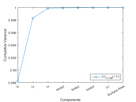
The current dataset can be described incredibly well just by looking at Iz, which again the models are rotated so that Iz is the largest moment of inertia. Then including Iy and Iz means that a 3D plot of the principle moments of inertia almost capture all the variation in the data.
The next step for characterization is to get only the inertia’s from the dataset. Since the current dataset is so small, the scaled dataset will be used for rest of the characterization process. Once more parts are added to the database it will make sense to start looking at the raw dataset. Now we can proceed to cluster the data using the k-means method of clustering. To properly use k-means a value of k, which is the number of clusters, needs to be determined. This can be done by creating an elbow plot using the following code:
for ii=1:20
    [idx,~,sumd] = kmeans(inertia,ii);
    J(ii)=norm(sumd);
end
Which produces the following plot:
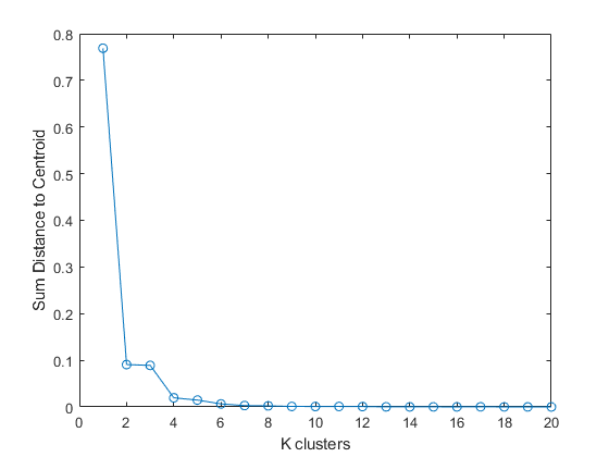
As can be seen in the above elbow plot, at 6 clusters there is an “elbow” which is where there is a large drop in the sum distance to the centroid of each cluster which means that it is the optimal number of clusters. The inertia’s can then be plotted using 6 k-means clusters produces the following plot:
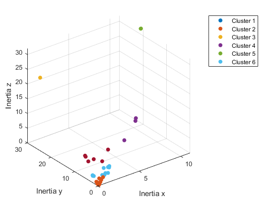
From this plot it is immediately clear that there are clusters of outliers. These are due to the different shapes and the extreme values are slender rods or flat plates while the clusters closer to the center more closely resemble a sphere. As the dataset grows it should become more apparent what kind of clusters actually make up a satellite, and eventually space debris in general.
Next Steps
The current dataset needs to be grown in both the amount of data and the variety of data. The most glaring issue with the current dataset is the lack of any debris since the parts are straight from satellite assemblies. Getting accurate properties from the current scans we have is an entire research project in itself, so hopefully, getting pieces that are easier to scan can help bring the project back on track. The other and harder-to-fix issue is finding/deriving more data properties. Properties such as cross-sectional or aerodynamic drag would be very insightful but are likely to be difficult to implement in code and significantly more resource intensive than the current properties the code can derive.