Anson’s Projects - Machine Learning Directed Study: Report 1

Gathering Data

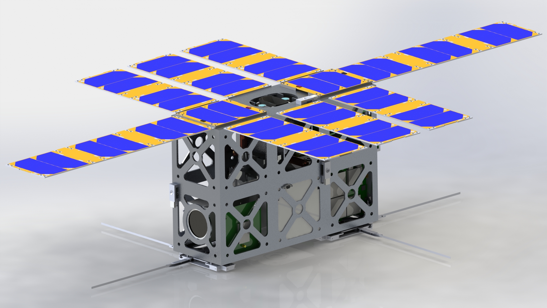
To get started on the project before any scans of the actual debris are made available, I opted to find similar 3D models online and process them as if they were data collected by my team. GrabCad is an excellent source of high-quality 3D models, and all of the models have at worst a non-commercial license making them suitable for this study. To start, I downloaded a high-quality model of a 6U CubeSat, which coincidentally enough was designed to detect orbital debris. This model consists of 48 individual parts, most of which are unique.

Data Preparation

To begin analysis of the satellite, fundamental properties from each piece needed to be derived. The most accessible CAD software for me is Fusion 360, but almost any CAD software can give properties for a model. The only way to export the properties from fusion is to my computer’s clipboard. This creates a long process that requires clicking on each part of the CubeSats assembly, then creating a text file and pasting my clipboard to the file. This task was easily automated using an AutoHotkey script to automatically push my computer’s clipboard to a file. Below is an example of each file’s contents, but only a portion of the file for brevity. The text file is generated in a way that makes it difficult to parse, so a separate piece of code was used to collect all of the data from all of the part files and then turn it into a .csv file for easy import into Matlab.

...
Physical
    Mass    108.079 g
    Volume  13768.029 mm^3
    Density 0.008 g / mm^3
    Area    19215.837 mm^2
    World X,Y,Z 149.00 mm, 103.80 mm, 41.30 mm
    Center of Mass  101.414 mm, 102.908 mm, -0.712 mm
...

The entire file of the compiled parts properties from Fusion 360 can be seen here. This method gave 22 columns of data, but most of the columns are unsuitable for the characterization of 3D geometry. The only properties considered must be scalars independent of a model’s position orientation in space. Part of the data provided was a moment of inertia tensor. The tensor was processed down to \(I_x\), \(I_y\), and \(I_z\), which was then used to calculate an \(\bar{I}\). Then bounding box length, width, and height were used to compute the total volume that the object takes up. In the end, the only properties used in the analysis of the parts were: mass, volume, density, area, bounding box volume, \(\bar{I}\), and material. Some parts also had to be removed because the final dataset is 44 rows and 7 columns. Below is a Splom plot which is a great way to visualize data of high dimensions. As you can see, most of the properties correlate with one another.

View Plot as an image

Now that the data is processed and clean, characterization in Matlab can begin. The original idea was to perform PCA, but the method had difficulties producing meaningful results. This is likely because the current dataset is tiny for machine learning and the variation in the data is high. The application of PCA will be revisited once the dataset grows. The first step for characterization is importing our data into Matlab.

data = readmatrix('prepped.csv');

Next k-means will be used to cluster the data. Since it is hard to represent data in higher dimensions than two, only two columns of data will be provided for the clustering. For now, I think it makes most intuitive sense to treat volume and mass as the most critical columns since the volume vs. mass plot shows 3 reasonably distinct groups.

[idx,C] = kmeans(data(:,1:2),3);

We can look at the distribution of parts in each cluster to ensure that each cluster has at least a few data points. Since k-means is an iterative method that relies on a user guess and randomness, it’s essential to ensure that the clusters make some sense.

histcounts(idx) =

    22    13     9

Then plotting Volume vs. Mass using our clusters produces the following plot. These make intuitive sense, but it is clear that the dataset needs much more data for Cluster 3.

Volume and Mass clusters

Below is another Splom, but with the clusters found above. Since the k-means only used Mass and Volume to develop its clusters, some of the properties do not cluster well against each other. This is also a powerful cursory glance at what properties are correlated.

View Plot as an image

Next Steps

The current dataset needs to be grown in both the amount of data and the variety of data. The most glaring issue with the current dataset is only two different material types. Modern satellites, and therefore their debris, is composed of dozens of unique materials. The other and harder to fix issue is finding/deriving more data properties. Properties such as cross-sectional are or aerodynamic drag would be very insightful, but there is no good way to collect that data. Thankfully, the 3D scanner methods to obtain more properties can be developed and applied over the entire dataset.

Once the dataset is grown, more advanced analysis can begin. PCA is the current goal and can hopefully be applied by the next report.

Check out the repo for this report for all the code and raw data. https://gitlab.com/orbital-debris-research/directed-study/report-1

Reuse

CC BY 4.0